Poker-Hand Prediction
Through this article I will try to show how can various classification algorithms be used to predict the possible poker-hand(s).
What is a “Poker-Hand” ?
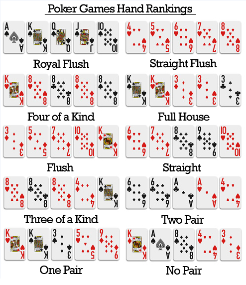
In poker, players structure sets of five cards, called hands, as per the principles of the game. Each hand has a position, which is looked at against the positions of different hands taking an interest in the standoff to choose who wins the pot.


DATA SET DESCRIPTION
Each record is an example of a hand consisting of five playing cards drawn from a standard deck of 52. Each card is described using two attributes (suit and rank), for a total of 10 predictive attributes. There is one Class attribute that describes the “Poker Hand”. The order of cards is important, which is why there are 480 possible Royal Flush hands as compared to 4 .
POKER-HAND DATA SET SOURCE : http://archive.ics.uci.edu/ml/machine-learning-databases/poker/
Data Set Attribute Description:
- S1 “Suit of card #1”
Ordinal (1–4) representing {Hearts, Spades, Diamonds, Clubs}
2) C1 “Rank of card #1”
Numerical (1–13) representing (Ace, 2, 3, … , Queen, King)
3) S2 “Suit of card #2”
Ordinal (1–4) representing {Hearts, Spades, Diamonds, Clubs}
4) C2 “Rank of card #2”
Numerical (1–13) representing (Ace, 2, 3, … , Queen, King)
5) S3 “Suit of card #3”
Ordinal (1–4) representing {Hearts, Spades, Diamonds, Clubs}
6) C3 “Rank of card #3”
Numerical (1–13) representing (Ace, 2, 3, … , Queen, King)
7) S4 “Suit of card #4”
Ordinal (1–4) representing {Hearts, Spades, Diamonds, Clubs}
8) C4 “Rank of card #4”
Numerical (1–13) representing (Ace, 2, 3, … , Queen, King)
9) S5 “Suit of card #5”
Ordinal (1–4) representing {Hearts, Spades, Diamonds, Clubs}
10) C5 “Rank of card 5”
Numerical (1–13) representing (Ace, 2, 3, … , Queen, King)
11) CLASS “Poker Hand”
Ordinal (0–9)
TYPES OF POKER HANDS:
0: Nothing in hand; not a recognized poker hand
1: One pair; one pair of equal ranks within five cards
2: Two pairs; two pairs of equal ranks within five cards
3: Three of a kind; three equal ranks within five cards
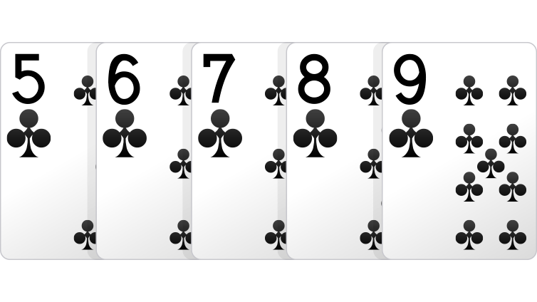
4: Straight; five cards, sequentially ranked with no gaps
5: Flush; five cards with the same suit
6: Full house; pair + different rank three of a kind
7: Four of a kind; four equal ranks within five cards
8: Straight flush; straight + flush
9: Royal flush; {Ace, King, Queen, Jack, Ten} + flush
IMPORTING ALL THE LIBRARIES
import pandas as pd
import numpy as np
import matplotlib.pyplot as plt
import warnings
warnings.filterwarnings('ignore')
DATA PRE-PROCESSING
data_train=pd.read_csv("poker-hand-training-true.data",header=None)
data_test = pd.read_csv("poker-hand-testing.data",header=None)
col=['Suit of card #1','Rank of card #1','Suit of card #2','Rank of card #2','Suit of card #3','Rank of card #3','Suit of card #4','Rank of card #4','Suit of card #5','Rank of card 5','Poker Hand']data_train.columns=col
data_test.columns=coly_train=data_train['Poker Hand']
y_test=data_test['Poker Hand']
y_train=pd.get_dummies(y_train)
y_test=pd.get_dummies(y_test)x_train=data_train.drop('Poker Hand',axis=1)
x_test=data_test.drop('Poker Hand',axis=1)print('Shape of Training Set:',x_train.shape)
print('Shape of Testing Set:',x_test.shape)>>Shape of Training Set: (25010, 10)
>>Shape of Testing Set: (1000000, 10)
1.NEURAL NETWORK
A neural network is a progression of algorithms that attempts to perceive fundamental connections in a lot of information through a procedure that copies the manner in which the human brain works. Neural network can adjust to changing input; so the network produces the most ideal outcome without expecting to redesign the output criteria.
To create NN we used Keras library which is a high-level API wrapper for the low-level API, capable of running on top of TensorFlow, CNTK, or Theano.
My neural network architecture comprised of 3 dense layers with respectively 15,10 and 10 nodes in each layer.
import keras
from keras.models import Sequential
from keras.layers import Dense, Dropout, Activation
from keras.optimizers import SGD
from keras import regularizers


model = Sequential()
model.add(Dense(15, activation='relu', input_dim=10))
model.add(Dense(10, activation='relu'))
model.add(Dense(10, activation='softmax'))
model.compile(loss='binary_crossentropy',
              optimizer='adam',
              metrics=['accuracy'])


history = model.fit(x_train, y_train, epochs = 10, batch_size = 256, verbose=1,validation_data=(x_test,y_test),shuffle=True)


score = model.evaluate(x_test, y_test, batch_size=256)##OUTPUTTrain on 25010 samples, validate on 1000000 samples
Epoch 1/10
25010/25010 [==============================] - 4s 156us/step - loss: 0.3935 - acc: 0.8842 - val_loss: 0.3070 - val_acc: 0.8999
Epoch 2/10
25010/25010 [==============================] - 4s 147us/step - loss: 0.2283 - acc: 0.8996 - val_loss: 0.1818 - val_acc: 0.8997
Epoch 3/10
25010/25010 [==============================] - 4s 145us/step - loss: 0.1790 - acc: 0.8998 - val_loss: 0.1767 - val_acc: 0.9000
Epoch 4/10
25010/25010 [==============================] - 4s 143us/step - loss: 0.1758 - acc: 0.9001 - val_loss: 0.1750 - val_acc: 0.9001
Epoch 5/10
25010/25010 [==============================] - 4s 149us/step - loss: 0.1748 - acc: 0.9000 - val_loss: 0.1743 - val_acc: 0.9000
Epoch 6/10
25010/25010 [==============================] - 4s 144us/step - loss: 0.1743 - acc: 0.9001 - val_loss: 0.1740 - val_acc: 0.9000
Epoch 7/10
25010/25010 [==============================] - 4s 146us/step - loss: 0.1740 - acc: 0.9003 - val_loss: 0.1737 - val_acc: 0.9001
Epoch 8/10
25010/25010 [==============================] - 4s 147us/step - loss: 0.1738 - acc: 0.9002 - val_loss: 0.1734 - val_acc: 0.9000
Epoch 9/10
25010/25010 [==============================] - 4s 146us/step - loss: 0.1735 - acc: 0.9005 - val_loss: 0.1732 - val_acc: 0.9003
Epoch 10/10
25010/25010 [==============================] - 4s 151us/step - loss: 0.1734 - acc: 0.9004 - val_loss: 0.1730 - val_acc: 0.9004
1000000/1000000 [==============================] - 3s 3us/step
Validation accuracy is coming out to be 90.04% .

Now experimenting and comparing with other classification models…
2.LOGISTIC REGRESSION
Like all regression analyses, the logistic regression is a predictive analysis. Logistic regression is used to describe data and to explain the relationship between one dependent binary variable and one or more nominal, ordinal, interval or ratio-level independent variables.
I used the Sci-kit Learn Library to import all algorithms and employed the Logistic Regression method of model selection to use Logistic Regression Algorithm.
from sklearn.linear_model import LogisticRegression
from sklearn.metrics import accuracy_score
clf = LogisticRegression(random_state=0, solver='lbfgs',max_iter=100,multi_class='ovr').fit(x_train, y_train)
y_pred=clf.predict(x_test)
accuracy_score(y_pred,y_test)##OUTPUT0.501209
As you can see the validation accuracy is surprisingly low as compared to that of Neural Network.
Validation accuracy is 50.12%!!
3.Classification And Regression Trees for Machine Learning(CART)
Classification and Regression Trees or CART for short is a term introduced by Leo Breiman to refer to Decision Tree algorithms that can be used for classification or regression predictive modeling problems.
Classically, this algorithm is referred to as “decision trees”, but on some platforms like R they are referred to by the more modern term CART.
The CART algorithm provides a foundation for important algorithms like bagged decision trees, random forest and boosted decision trees.
I used the Sci-kit Learn Library to import all algorithms and employed the Decision Tree method of model selection to use Decision Tree Algorithm.
from sklearn.tree import DecisionTreeClassifier
decision_tree = DecisionTreeClassifier(random_state=0,max_depth = 2)
decision_tree = decision_tree.fit(x_train,y_train)
y_pred = decision_tree.predict(x_test)
accuracy_score(y_pred,y_test)##OUTPUT0.501209
Again the validation accuracy is surprisingly low and is very similar to that of Logistic Regression
Validation accuracy is 50.12%!!
AND FINALLY…
4.Support Vector Machine(SVM)
SVM is a supervised machine learning algorithm which can be used for both classification or regression challenges. However, it is mostly used in classification problems. In this algorithm, we plot each data item as a point in n-dimensional space (where n is number of features you have) with the value of each feature being the value of a particular coordinate.
from sklearn import svm
clf = svm.LinearSVC()
clf.fit(x_train,y_train)
y_pred = clf.predict(x_test)
accuracy_score(y_pred,y_test)##OUTPUT0.431699
The validation accuracy achieved here is 43.16%!
HERE IS MY COMPLETE CODE:
In the end, the Neural Network using Keras Library enables us to produce the most accurate results above all!
This is one of my first applications in machine learning. Thank you for reading my article, and I hope I was able to help and inspire students like myself!